Procedures and strategy for estimating the systematics uncertainties¶

Setting it up¶

If you have done the fitting tutorial you already have done this part so you may go directly to "Generating uncertainties" Clone this repository and go to the fitting folder.

git clone git://github.com/cms-legacydata-analyses/TagAndProbeTool
cd TagAndProbe/efficiency_tools/fitting

You will also need to download the Run2011AMuOnia_mergeNtuple.root file using this link.

https://cernbox.cern.ch/index.php/s/lqHEasYWJpOZsfq

Data simplifying¶

In order to run this code, use this command to simplify the data so that it can be read by the RooFit root library.

root simplify_data.cpp

This will create a "TagAndProbe_Jpsi_Run2011.root" file, this process may take a few minutes. move the file to the DATA folder.

Estimations of systematics uncertainty sources¶

To estimate the systematic error we will need first to get some uncertainties from the DATA. So, to do that, run the following code.

root -l -b -q plot_sys_efficiency.cpp

By default, this code will estimate the Muon ID efficiency for the Global Muon ID for |η| distribution, this can be changed by opening the "plot_sys_efficiency.cpp" and commenting and uncommenting the Muon ID and quantity of your desire. This process may take several minutes to complete.

The systematics uncertainties will be evaluate by making small changes in the fit on the invariant mass distribution of the resonance. For example, the ψ decaying in dimuons, in this case the changes were: 2x Gaussians ("2x gaus" as in the code) which means fitting with two gaussians. The other sources are the upper and under limits of invariant mass distribution and so "Mass Up" which means making the mass window bigger, "Mass Down" which means making the mass window smaller. Last source you can modify the bin size of the same distribution. "Bin up" means making the fit with more bins and "Bin down" means making the fit with less bins.

In order to do the next step you will have to run the "plot_sys_efficiency.cpp" for the Pt of both global and tracker Muon. To get the Pt for the traker Muons the code should look like this.

//Which Muon Id do you want to study?
string MuonId   = "trackerMuon";
//string MuonId   = "standaloneMuon";
//string MuonId   = "globalMuon";

//Which quantity do you want to use?
string quantity = "Pt";     double bins[] = {0., 3.0, 3.6, 4.0, 4.4, 4.7, 5.0, 5.6, 5.8, 6.0, 6.2, 6.4, 6.6, 6.8, 7.3, 9.5, 13.0, 17.0, 40.};
//string quantity = "Eta";    double bins[] = {-2.4, -1.4, -1.2, -1.0, -0.8, -0.5, -0.2, 0, 0.2, 0.5, 0.8, 1.0, 1.2, 1.4, 2.4};
//string quantity = "Phi";    double bins[] = {-3.0, -1.8, -1.6, -1.2, -1.0, -0.7, -0.4, -0.2, 0, 0.2, 0.4, 0.7, 1.0, 1.2, 1.6, 1.8, 3.0};

//string quantity = "Pt";     double bins[] = {0.0, 2.0, 3.4, 4.0, 5.0, 6.0, 8.0, 10.0, 40.};
//string quantity = "Eta";    double bins[] = {0.0, 0.4, 0.6, 0.95, 1.2, 1.4, 1.6, 1.8, 2.4};

and like this to the global Muons.

//Which Muon Id do you want to study?
//string MuonId   = "trackerMuon";
//string MuonId   = "standaloneMuon";
string MuonId   = "globalMuon";

//Which quantity do you want to use?
string quantity = "Pt";     double bins[] = {0., 3.0, 3.6, 4.0, 4.4, 4.7, 5.0, 5.6, 5.8, 6.0, 6.2, 6.4, 6.6, 6.8, 7.3, 9.5, 13.0, 17.0, 40.};
//string quantity = "Eta";    double bins[] = {-2.4, -1.4, -1.2, -1.0, -0.8, -0.5, -0.2, 0, 0.2, 0.5, 0.8, 1.0, 1.2, 1.4, 2.4};
//string quantity = "Phi";    double bins[] = {-3.0, -1.8, -1.6, -1.2, -1.0, -0.7, -0.4, -0.2, 0, 0.2, 0.4, 0.7, 1.0, 1.2, 1.6, 1.8, 3.0};

//string quantity = "Pt";     double bins[] = {0.0, 2.0, 3.4, 4.0, 5.0, 6.0, 8.0, 10.0, 40.};
//string quantity = "Eta";    double bins[] = {0.0, 0.4, 0.6, 0.95, 1.2, 1.4, 1.6, 1.8, 2.4};

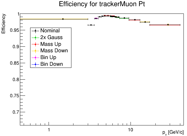
Systematic efficiency overplot¶

To better understand the results of the last part, this code will put all the different plots created previously in an image.

root overplot_efficiencies.cpp

You should get a result like this:

Efficiency Systematic Overplot 1D

2D Efficiency Map¶

This code generates a 2D systematic efficiency overplot, it outputs a .root that contains the efficiency histograms that can be visualised by the root TBrowser.

root -l -b -q plot_sys_efficiency_2d.cpp

This is one of the graphs that will be generated.

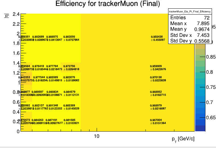
Efficiency Systematic Overplot 2D

It is noteworthy that the uncertainties presented above in the 2d map are already the quadrature sum of systematics and statistical uncertainties.