How to make a comparison between two previous methods of signal extraction

How sideband subtraction method code stores its files

the Sideband subtraction code saves every efficiency plot in efficiency/plots/ folder inside a single generated_hist.root file. Lets check it!

You're probably on the main directory. Lets go back one directory.

cd ..
ls

JPsiToMuMu_mergeMCNtuple.root  README.md  Run2011AMuOnia_mergeNtuple.root
main                           results

A folder named results showed up on this folder. Lets go check its content.

cd results
ls

Jpsi_MC_2020  Jpsi_Run_2011

If you did every step of the sideband subtraction on this page lesson, these results should match with the results on your pc. Access one of those folders (except comparison).

cd Jpsi_Run_2011
ls

Efficiency_Tracker_Probe_Eta.png  Tracker_Probe_Eta_All.png
Efficiency_Tracker_Probe_Phi.png  Tracker_Probe_Eta_Passing.png
Efficiency_Tracker_Probe_Pt.png   Tracker_Probe_Phi_All.png
generated_hist.root               Tracker_Probe_Phi_Passing.png
InvariantMass_Tracker.png         Tracker_Probe_Pt_All.png
InvariantMass_Tracker_region.png  Tracker_Probe_Pt_Passing.png

Here, all the output plots you saw when running the sideband subtraction method are stored as a .png. Aside from them, there's a generated_hist.root that stores the efficiency in a way that we can manipulate it after. This file is needed to run the comparison between efficiencies for the sideband subtraction method. Lets look inside of this file.

Run this command to open generated_hist.root with ROOT:

root -l generated_hist.root

root [0]
Attaching file generated_hist.root as _file0...
(TFile *) 0x55dca0f04c50
root [1]

Lets check its content. Type on terminal:

new TBrowser

You should see something like this:

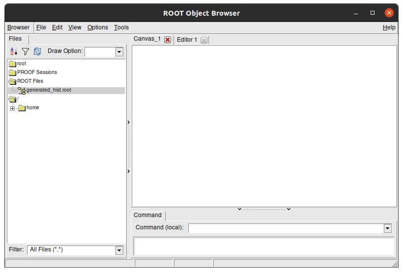
This is a visual navigator of a .root file. Here you can see the struture of generated_hist.root. Double click the folders to open them and see their content. The Efficiency plots we see are stored in efficiency/plots/ folder:

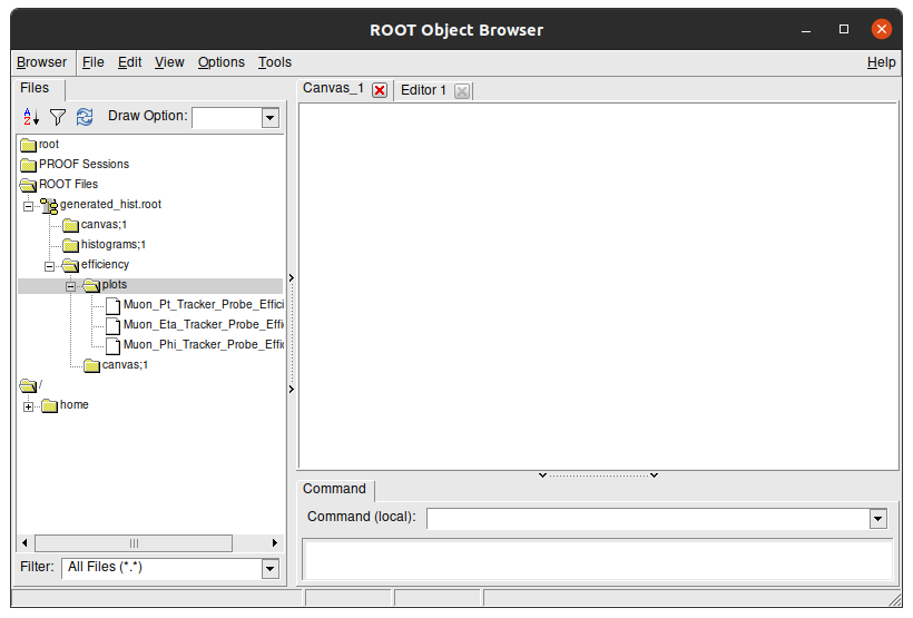
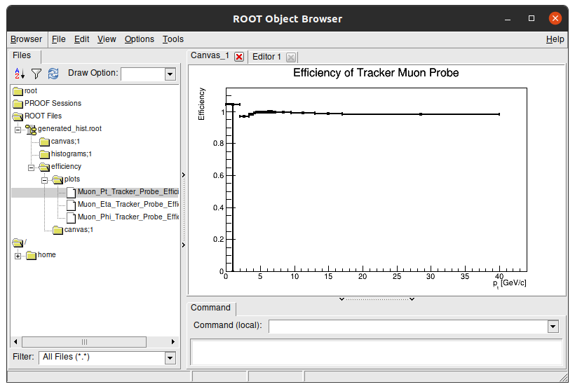
You can double click each plot to see its content:

Tip

To close this window, click on terminal and press Ctrl + C. This command stops any processes happening in the terminal.

Key Point

• As you see, the .root file has paths inside of it and the efficiencies plots have a self path inside them as well!

Comparison results between real data and simulations for sideband method

After runinng the sideband subtraction code, we get a .root with all the efficiencies plots inside it in two different folders:

• ../results/Jpsi_Run_2011/generated_hist.root
• ../results/Jpsi_MC_2020/generated_hist.root

We'll get back to this on the discussion below.

Head back to the main folder. Inside of it there is a code for the efficiency plot comparison. Lets check it out. From the sideband_subtraction folder, type:

cd main
ls

classes  compare_efficiency.cpp  config  macro.cpp

There is it. Now lets open it.

gedit compare_efficiency.cpp

Its easy to prepare it for the sideband subtraction comparison. Our main editing point can be found in this part:

//CONFIGS

int useScheme = 0;
//Jpsi    Sideband Run vs Jpsi    Sideband MC
//Jpsi    Fitting  Run vs Jpsi    Fitting  MC
//Jpsi    Sideband Run vs Jpsi    Fitting  Run
//Upsilon Sideband Run vs Upsilon Sideband MC
//Upsilon Fitting  Run vs Upsilon Fitting  MC
//Upsilon Sideband Run vs Upsilon Fitting  Run

//Muon id analyse
bool doTracker    = true;
bool doStandalone = true;
bool doGlobal     = true;

//quantity analyse
bool doPt  = true;
bool doEta = true;
bool doPhi = true;

Note

In the scope above we see:

• int useScheme represents which comparison you are doing.
• bool doTracker is a variable that allow plots for tracker muons.
• bool doStandalone is a variable that allow plots for standalone muons.
• bool doGlobal is a variable that allow plots for global muons.
• bool doPt is a variable that allow plots for muon pT.
• bool doEta is a variable that allow plots for muon η.
• bool doPhi is a variable that allow plots for muon φ.

Everything is up to date to compare sideband subtraction's results between real data and simulations, except it is comparing standalone and global muons. As we are looking for tracker muons efficiencies only, you should switch to false variables for Standalone and Global.

Also, you will need to change the useScheme variable to plot what you want to plot. As we want to plot efficiency of real data and simulated data, the value has to be 0.

See result scructure

If you deleted the right lines, your code now should be like this:

//CONFIGS

int useScheme = 0;
//Jpsi    Sideband Run vs Jpsi    Sideband MC
//Jpsi    Fitting  Run vs Jpsi    Fitting  MC
//Jpsi    Sideband Run vs Jpsi    Fitting  Run
//Upsilon Sideband Run vs Upsilon Sideband MC
//Upsilon Fitting  Run vs Upsilon Fitting  MC
//Upsilon Sideband Run vs Upsilon Fitting  Run

//Muon id analyse
bool doTracker    = true;
bool doStandalone = false;
bool doGlobal     = false;

//quantity analyse
bool doPt  = true;
bool doEta = true;
bool doPhi = true;

Let your variables like this.

Now you need to run the code. To do this, save the file and type on your terminal:

root -l compare_efficiency.cpp

If everything went well, the message you'll see in terminal at end of the process is:

Use Scheme: 0
Done. All result files can be found at "../results/Comparison_Upsilon_Sideband_Run_vs_MC/"

Note

The command above to run the code will display three new windows on your screen with comparison plots. You can avoid them by running straight the command below.

root -l -b -q compare_efficiency.cpp

In this case, to check it results you are going to need go for result folder (printed on code run) and check images there by yourself. You can try to run new TBrowser again:

cd [FOLDER_PATH]
root -l
new TBrowser

And as output plots comparison, you get:

Now you can type the command below to quit root and close all created windows:

.q

How fitting method code stores its files

To do the next part, first you need to understand how the fitting method code saves. It is not so different than sideband subtraction method. Lets look at how they are saved.

If you look inside fitting\results' folder, where is stored fitting method results, you will see another folder named efficiencies. lets go there by terminal from fitting folder:

cd results/efficiencies
ls

efficiency

Inside of it there is a unique folder named efficiency. It is necessary because later on, we will work in efficiencies in 2 dimentions. The efficiency folder means it is one-dimensional, which we worked here so on.

cd efficiency
ls

Comparison_Run2011_vs_MC  Jpsi_MC_2020  Jpsi_Run_2011

Let's go inside one of them:

cd Jpsi_Run_2011
ls

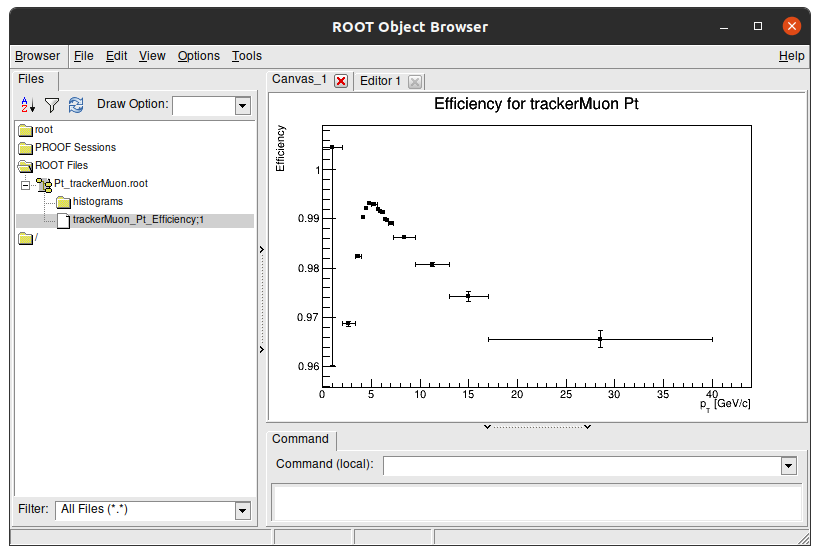
Pt_trackerMuon.root

For every configuration for a specific dataset, they will create .root files inside its respectively folder. For example, this one folder that we choose will have all calculations for the J/ψ real data dataset.

If you go with your terminal to this folder and run this command, you'll see that the result files only have one plot on main folder.

root -l Pt_trackerMuon.root

root [0]
Attaching file Pt_trackerMuon.root as _file0...
(TFile *) 0x55efb5f44930
root [1]

Now lets look at its content. Type on terminal:

new TBrowser

It has only one plot, because the others are in different files. Inside the folder histograms, you can find the histograms that created this efficiency result.

Key Point

• There is a .root file for each efficiency plot created with the fitting method.

Comparison results between real data and simulations for fitting method

Go back to the main folder on sideband_subtraction folder.

cd main
ls

classes  compare_efficiency.cpp  config  macro.cpp

Open compare_efficiency.cpp again

gedit compare_efficiency.cpp

This is how your code should look like now:

//CONFIGS

int useScheme = 0;
//Jpsi    Sideband Run vs Jpsi    Sideband MC
//Jpsi    Fitting  Run vs Jpsi    Fitting  MC
//Jpsi    Sideband Run vs Jpsi    Fitting  Run
//Upsilon Sideband Run vs Upsilon Sideband MC
//Upsilon Fitting  Run vs Upsilon Fitting  MC
//Upsilon Sideband Run vs Upsilon Fitting  Run

//Muon id analyse
bool doTracker    = true;
bool doStandalone = false;
bool doGlobal     = false;

//quantity analyse
bool doPt  = true;
bool doEta = true;
bool doPhi = true;

You have to do just two things:

1. edit int useScheme value to current analysis.

2. Put others quantities expect pT to false, we did not obtained η nor φ results on previous page.

After making those edits

Your code should look like this:

//CONFIGS

int useScheme = 1;
//Jpsi    Sideband Run vs Jpsi    Sideband MC
//Jpsi    Fitting  Run vs Jpsi    Fitting  MC
//Jpsi    Sideband Run vs Jpsi    Fitting  Run
//Upsilon Sideband Run vs Upsilon Sideband MC
//Upsilon Fitting  Run vs Upsilon Fitting  MC
//Upsilon Sideband Run vs Upsilon Fitting  Run

//Muon id analyse
bool doTracker    = true;
bool doStandalone = false;
bool doGlobal     = false;

//quantity analyse
bool doPt  = true;
bool doEta = false;
bool doPhi = false;

Doing this and running the program with:

root -l compare_efficiency.cpp

Should get you these results:

Challenge

As you notice here we presented comparison for η and φ. Try to go back to fitting method tutorial and redo commands to get efficiencies for these quantities in order to compare with sideband subctraction method. Do not forget to turn bool doEta and bool doPhi true.

Now you can type the command below to quit root and close all created windows:

.q

Comparison results between data from the sideband and data from the fitting method

Challenge

Using what you did before, try to mix them and plot a comparison between real data for sideband method and real data for sthe fitting method and get an analysis. Notice that:

• Real data = Run 2011
• Simulations = Monte Carlo = MC

Tip: you just need to change what you saw in this page to do this comparison.

---

Extra challenge

As you did with the last 2 extras challenges, try to redo this exercise comparing results between Υ datas.